Tejas Mohan Ayyar

Classification of Animals in the wild using CNN models and Tensorflow (Keras)

I started learning about Neural Networks and different model architectures in CNN. Here I am writing about 4 model architectures and what were my findings when I trained my image set on these 4 models. The article was written for learning purpose only and to get a better understanding of the improvements we see across these models.

All observations here are tied to one image set and cannot be taken as a metric for how well a model performs. It depends on each use case as to which model would be best suited. For example if you read about my metal casting project, a simple CNN model tended to do much better than the ResNet model which performs brilliantly here.

Dataset used for the experiment

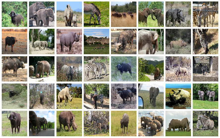
I have used the African wildlife dataset for my experiment.

There are 4 classes in this dataset:

• Buffalo
• Elephant
• Rhino
• Zebra

Contents of this article:

• What are Convolutional Neural Networks
• Implementing 4 different CNN models on the mentioned dataset and giving a brief of each model with inferences from my experiment.
• Conclusions

What are Convolution Neural Networks?

• A Convolutional Neural Network is a type of artificial neural network that is primarily used for image recognition applications. It consists of multiple layers called perceptrons for learning features present in images with utmost detail.

• “Convolution” here represents the understanding of features within an image. Extracting these features entails the entire process of convolution.

• To extract these features we use filters and mention the number of filters to be used (Kernels).

• Pooling is another concept in CNN. It is used to reduce the number of features that we get after we have run our filters over the images. The filters cause us to get a large number of features compared to the image itself. So pooling is used to get a better generalized representation of the same. For example a 25x25 image might end up with 100x100 features due to the number of filters (kernels) and their shape. Pooling can reduce these features either using max pooling or mean pooling. I will not delve much into what pooling is.

• Padding is another CNN concept where we add zeros to the edges of an image. This is done for 2 reasons. To better read the edge features and to get similar output as the input image.

• Lastly the output of the CNN is flattened and sent into a fully connected layer. This is our Neural Network part of CNN. It will enable the machine to learn from the extracted features and create a generalized model.

• To know more about Convolutional Neural Networks I would start from this video.

4 model architectures used in the experiment and their inferences.

LeNet

• The LeNet architecture was invented in 1998 by Yann Lecun with the aim to be able to perform Optical Character Recognition (OCR). The architecture is very small and simple compared to other architectures. The image set consisted of images of numbers from 0-9 in black and white.

• It consists of 3 convolution layers and 3 pooling layers. After these layers the outputs are flattened and the data is sent into a Fully connected layer. The last dense layer of the Neural Network can be any activation function for predicting the output.

• Across the entire network according to the paper published for LeNet, activation functions across all the layers were tanh. I have used the same activation function for this network. We have to remember that the commonly used activation functions used today were not there in 1998.

Implementation in your example and your findings

• As can be observed from the above graph of accuracy, we can clearly see the slow learning rate that this model is displaying.
• There could be many reasons for this.
• The lack of depth of this network is one reason.
• Another reason could be the activation function tanh which has been used.

Advantages

• This network was a good introduction into the world of neural networks and is really simple to understand. It works well for character recognition images.

Disadvantages

• This model was more specifically built for a certain use case. While it was a major breakthrough in 1998, it does not do as well with color images. Most image recognition problems would require RGB images for better recognition.

• Since the model isn’t very deep, it struggles to scan for all features thus producing poor performing models. If the Neural Network isn’t fed with enough features from the training images then it would be difficult for the model to generalize and create an accurate model.

AlexNet

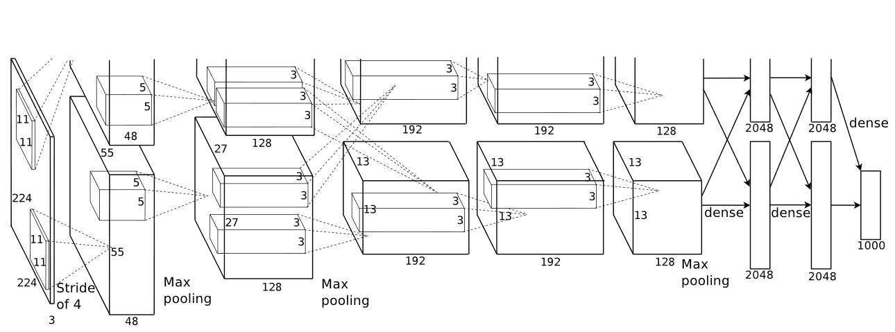
• The AlexNet architecture was introduced in 2012 at the ImageNet Large Scale Visual Recognition Challenge.
• It was designed by Alex Krizhevsky and published with Illya Sutskever and Krizhevsky’s doctoral advisor Dr. Geoffrey Hinton.

• AlexNet consisted of 8 layers and used the ReLu activation function which was a major discovery in deep learning. It got rid of the vanishing gradient problem since now the gradient values were not limited to a certain range.

• It was the first GPU based CNN model and was 4 times faster than previous models.

Implementation in your example and your findings

• What I observed is that the speed of training improved when compared to LeNet. We clearly can see in the graph that this model achieves a better accuracy much faster.

• Loss also reduces at a faster rate when compared to LeNet.

• The increase in depth of the network and introduction of ReLu had a major impact in Neural Networks. This model inspired the research of future models.

Advantages

• AlexNet was the first major CNN model that used GPU’s for training. This lead to faster training of models.
• AlexNet is a deeper architecture with 8 layers which means that is better able to extract features when compared to LeNet. It also worked well for the time with color images.
• The ReLu activation function used in this network has 2 advantages. It does not limit the output unlike other activation functions. This means there isn’t too much loss of features.
• It negates the negative output of summation of gradients and not the dataset itself. This means that it will further improve model training speed since not all perceptrons are active.

Disadvantages

• Compared to models used further in this article, the depth of this model is very less and hence it struggles to learn features from image sets.

• We can see that it takes more time to achieve higher accuracy results compared to future models.

VGG

• Visual Geometric Group or VGG is a CNN architecture that was introduced 2 years after AlexNet in 2014. The main reason for introducing this model was to see the effect of depth on accuracy while training models for image classification/recognition.

• The VGG network introduced the concept of grouping multiple convolution layers with smaller kernel sizes instead of having one Conv layer with a large kernel size. This caused the number of features at the output to reduce and second was including 3 ReLu layers instead of one increasing learning instances. As can be seen from the image above we see the layered structure (grey boxes) followed by a pooling layer(red boxes).

Implementation in your example and your findings

• My observation here is that while the number of epoch’s required to achieve max accuracy has decreased, however the loss is taking much longer to converge to minima.

• The introduction of more layers in VGG has allowed the model to better understand the features within an image.

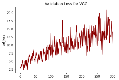
• However constantly learning and relearning is a problem with VGG which is why the loss seems to be so unpredictable (explosion of gradients).

• This problem is resolved in the ResNet architecture that introduces the concept of residual learning.

• Validation loss tends to increase overtime which tells me that this model was overfitting the dataset over time. This may not always be the case with other image sets.

Advantages

• VGG brought with it a massive improvement in accuracy and an improvement in speed as well. This was primarily because of improving the depth of the model and also introducing pretrained models.

• The increase in the number of layers with smaller kernels saw an increase in non-linearity which is always a positive in deep learning.

• VGG brought with it various architectures built on the similar concept. This gives more options to us as to which architecture could best fit our application.

Disadvantages

• One major disadvantage that I found was that this model experiences the vanishing gradient problem. If we look at my validation loss graph, we clearly see it increasing as a trend. This wasn’t the case with any of the other models. The vanishing gradient problem was solved with the ResNet architecture.

• VGG is slower than the newer ResNet architecture that introduced the concept of residual learning which was another major breakthrough.

*There is the Inception-V1 and Inception-V3 models that came in 2006 and 2008 as well but I have skipped those models from my experiment.

ResNet

• ResNet was introduced in 2015 and brought a massive improvement in accuracy and a major speed improvement.

• VGG had introduced the concept of increasing layers for better accuracy, however it was found that when we increase the number of layers beyond 20, the model is not able to converge to the minimum error %. A major reason for this is the vanishing gradient problem. learning rate becomes so less that there are no changes being introduced into the weights of the model.

• Another problem was the explosion of gradients. This is also visible in my VGG graph where my loss fluctuates erratically. This was solved when Batch Normalization was introduced but it still fluctuates albeit over a smaller range.

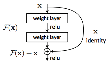
• To combat this, the concept of residual learning was introduced which was inspired from the concept of lateral inhibition in the human brain. It simply means that the neurons in the brain are able to control whether their neighbouring neurons fire or not.

• Residual learning can be explained with a very simple example. Initially when we learn to ride a bike we make mistakes and we learn. Once we are able to ride the bike, our brain has stopped fiering the neurons responsible to learn the skill allowing us to focus on other things involved with riding the bike.

Implementation in your example and your findings

• We see a drastic improvement in achieving high accuracy and low loss. The concept of residual learning can be called a major breakthrough in Neural Networks.

• The model created from the ResNet archtecture also had a low validation loss which meant that there was no overfitting happening while training.

Advantages

• The ResNet architecture does not need to fire all neurons in every epoch. This greatly reduces the training time and improves accuracy. Once a feature is learnt, it does not try to learn it again but rather focuses on learning newer features. A very smart approach that greatly improved model training performance.

• The complexity of an identical VGG network caused the degradation problem which was solved by residual learning.

Next Step

• Write front end for the web app.
• Deploy this on one of the cloud platforms like Heroku or GCP.

Conclusions

I performed this experiment to get a better understanding of the different types of model and how do they practically impact training of image classification models. You can further explore this experiment on my colaboratory notebook here. The images used are from this kaggle competition.

Thanks for reading!